The Computer Thinks We Would Be Friends

A crash course in Decision Tree Learning + a project I definitely didn't build out of insecurity

While on a long and boring train ride, I had a question I tend to have every so often: ‘Do People Like Me?’

The CMI Cat by Arushi Marwaha

Now unlike cats who famously don’t seem to have any kind of imposter syndrome, I do have my insecurities about if people are just too kind and if everyone just bears with me. It’s not really a pleasant question but one does wonder sometimes, especially on a long and boring train ride.

This naturally led to me asking: how do I decide if I like someone? Well, this also doesn’t seem to admit a clean answer. Liking someone is not some checklist after all, it’s more of a feeling.

This spiralled into me asking: Is there a way for me to make a quiz which can tell me if I’ll vibe with a person? Well, this sounds like a statistics or machine learning question and is more tractable.

Flow Chart Quizzes

If you grew up on a steady diet of magazines or were a Pinterest person, you might remember these kinds of flow chart personality tests.

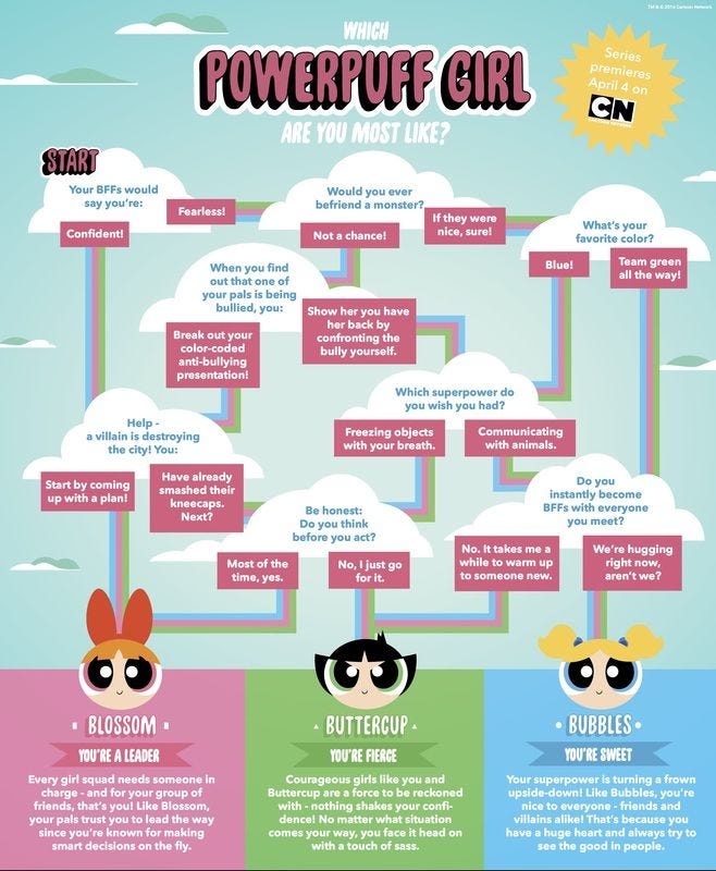
Now while these kind of personality tests are made rather subjectively by the whims of authors and their understanding of the characters defining traits, could we use data and math to make a more accurate version?

This was the question asked in 1950s concurrently by psychologists, statisticians and computer scientists. What followed was the theory of Decision Tree Learning.

Simple Decision Tree

From a different project¹, I had the responses of about 120 CMI people to a variety of questions about habits, beliefs, opinions and more. I also could simply go through the data and label if I vibe with a person or not.

So how would we go about making a flow chart quiz out of this dataset?

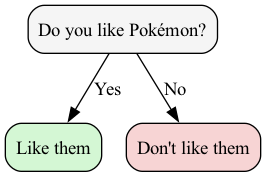
Let’s solve a simpler problem by going back to when I was in grade 3. At that point, I would vibe with anyone who loved Pokemon and dislike anyone who didn’t. Can you see how this would translate to a flowchart?

But say when I got to 4th grade, the people I knew and I both got a bit more complex. Now say asking the Pokemon question splits my acquaintances as: [1,5] and [5,1] while a question about enjoying the science classes splits them [2,0] and [4,6].

Which question is better now, given we can only ask 1? Someone could argue that it is the former as it classifies decently well while another person could argue that the second question is superior as a ‘yes’ guarantees we’ll be great friends.

How do we choose?

Well, one idea² is to choose the question that reduces the odds of misclassifying. Basically, given a random person, how often would I misclassify them?

Consider the pokemon question: If I look into the ‘yes’ bucket, a random person has probability 5/6 of being liked and 1/6 of disliked. So, if I pick a random person and classify them randomly (using the bucket’s distribution), I would be correct with odds 5/6 * 5/6 + 1/6* 1/6 = 26/36 and hence, wrong with odds 10/36. Same with the ‘no’ bucket. We can take the weighted average (i.e. multiply by the number of people in the bucket) and get an error rate of the question. In this case, 5/18 * 6/12 + 5/18 * 6/12 = 5/18.

Similarly, with the science question: we would have the yes bucket’s odds of error 0 and the no bucket’s odds 1 - (2/5 * 2/5 + 3/5 * 3/5) = 12/25. So, taking the weighted average, we get 0 * 2/12 + 12/25 * 10/12 = 2/5.

As 5/18 < 2/5, the error chance of the former question is lower and hence, using the Pokemon question is better.

This gives us a quantitative way to measure the usefulness of a question. This is called the Gini Index or Gini Impurity of a question and it ranges from 0 (perfect question) to 0.5 (as good as random).

A simple algorithm to generate a decision tree (aka a flow chart quiz) would be asking one good question after the another (note, different branches can have different questions!).³

So coming back to my problem at hand, my survey had about 60 statements and I had asked people to rate them from 1 (strongly disagree) to 10 (strongly agree). We can set each question as if you rated a particular statement above some threshold (so a total of 9*60 =540 choices of questions).

Finally, I keep aside a random fifth of the data set for predicting accuracy.

With all that said and done, we get the following tree:

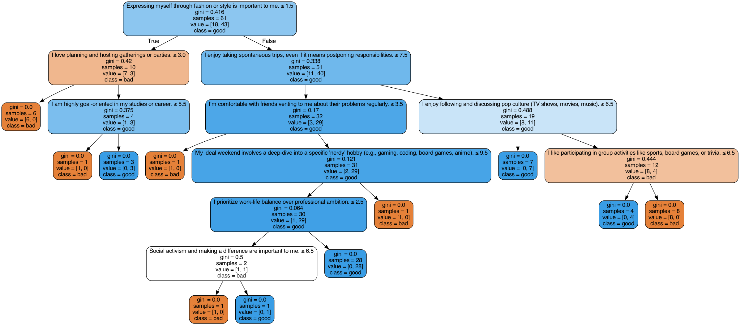
And this tree has an accuracy of 62%.

This might seem impressive for a rather simple algorithm, but it gets a lot less surprising if you consider the fact that the root (“Expressing myself through fashion or style is important to me”) gives a 58% accuracy.

Apart from the data outing me as something of a Miranda Priestly⁴, our tree is clearly not doing very well.

This is because of overfitting. Our tree on the 4/5th of the data it was created using has 100% accuracy. This means small changes in that data would make huge changes in this tree and hence, the tree is not robust aka it is too tightly based on the provided data.

So what should we do? Well, first we can restrict the depth of the tree to prevent it from going on and on. Next, we could say that every branch must have at least some number of candidates to prevent branches with just some 2-3 people. Finally, we can say every leaf must have some number of candidates to prevent leaves with a singular good or bad candidate.

How do we choose these parameters? I could actually sit and think about the data and do some statistics and choose them. Or, I could simply run the algorithm varying the parameters and choose the best.

The latter seems better as any statistics I do would bring more of methodological bias into the model. So trying all the parameters and choosing the best is sort of a neutral way.

However, we still need to be careful of coincidences. Some set of parameters could just be good on our 4/5th by sheer luck (and hence, the tree is not really going to perform that well in the wild).

So instead of choosing a 4/5th and then varying the parameters, we do it the other way around. We choose a set of parameters, then randomly choose a random 4/5th of the data to train on and use the remaining data to predict accuracy (and repeat this a few times and take average). This is called cross-validation.

So implementing all this, we get:

This has a 66% accuracy using the parameters 4 and 19 for minimum leaf size and minimum node size.

While it might seem that our previous discussion was much ado about nothing, notice that this is a much simpler tree and still has a better accuracy as it has made peace with being wrong on some nodes for a better accuracy.

But can we do better?

Decision Forests

Again, almost all of the error comes from overfitting, but this time we the problem is perhaps with the parameters. Notice, that our second tree doesn’t use the best question due to the choice of parameters.

Furthermore, 19 and 4 seem really weird as parameters as they seem quite large for our data of 120 people. This is probably happening due to the wide variety of questions.

So what can we do? Well, if the problem is too much information, let’s get rid of some of the information.

That probably sounds stupid as we are wasting data for questionable gains.

But we could simply remedy that make a bunch of trees (a forest) using different subsets of the dataset.

How do we classify something? We classify according to each of the trees and see the majority vote.

The only issue with this idea is that we can make about 2^60 * 2^120 (which is approximately 15 followed by 53 zeros) sub-datasets and even training at 1000 trees per second, it would take so long that even black holes won’t survive to see it. So as I am impatient, we will randomly choose some 100 of these sub-datasets (roughly of size sqrt of the original dataset) and make a random forest using them.

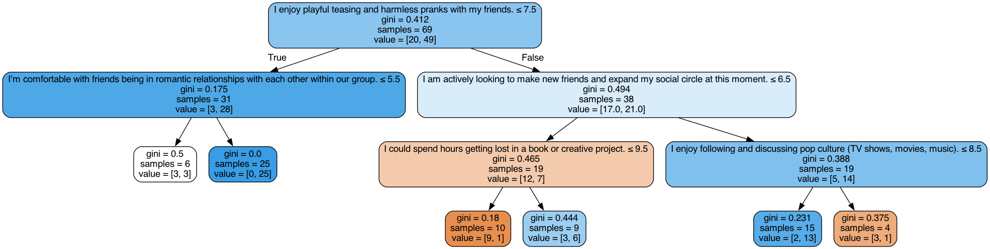
I would love to show you all the 100 trees but trying to cram them onto one image gave me a massive 18 MB image so I’ll instead show you 9 of them.

However, our accuracy is still around 66%

Why? Look at the trees. They are again committing the cardinal sin of overfitting on their datasets. Hence, we need to vary the parameters and use cross-validation.

As a result, we get the following nine tree forest with every node having size at least 8 and every leaf having size at least 9.

This has accuracy 69%. That’s great, we got a simpler model with higher accuracy.

However, the choice of the above parameters still seems alien. It is still highly dependent on the data. By democratising the process, we have made the overall model better but the individual trees are still not that good.

Gradient Boosted Trees

Instead of allowing individual trees to make full votes, let’s say we allow them to add or subtract from a score. If the score hits 0, it concludes that we won’t vibe and if it hits 1, it says the vibes will be crazy with them. We’ll start the score at 0.5.

This would allow the trees to be rather weak in some way, as in as long as they do better than random chance (even if slightly); we will eventually converge to the correct choice.

Let’s take a short detour to a party trick I had learned when I was in class 6. It was a math party trick so not many people found it cool but it happens to be rather useful in this case.

The setup was rather simple, I would ask someone to give upto a 4 digit number and I would predict the square root upto 2 decimal places almost instantly.

Let’s say one is to find the root of 62. We know that 8^2 = 64 so it has to be between 7 and 8. A bad answer would be to split the difference and say 7.5. We could perhaps square 7.5 and indeed, 56.25 is less than 62 so update our guess to 7.75, but this is still not very good. Although, if you could square 7.75, you could probably make a slightly better guess.

However, this algorithm ignores the fact that we are looking to find the square root. What I mean to say is the above algorithm (referred to as Binary Search) would work on cube roots and logs and well, any function that is increasing.

Perhaps, using the fact that we need to find the square root might help achieve a better approximation. Let’s guess the answer to be 8. Then, we can notice that 64-49 = 15, thus, we can update our guess to 8 - 2/15 = 7.867 which approximates to 7.87. This is quite good as the true value is 7.874.

We could repeat these steps indefinitely and get even better estimates.

Basically, √t ≈ √x + (x − t)/(x² − (√x − 1)²) = √x + (x − t)/(2√x + 1) ≈ √x + (x − t)/(2√x) where x is the nearest perfect square to t. So I used to just go to the nearest perfect square, subtract the target, divide the difference by twice the root of said perfect square and add the root of said perfect square.

Seems intuitive right? If you have done calculus, this probably rings some bells as 1/((2√x) is the derivative of √x - c where c is any constant, in this case t.

Basically, we can make a guess x and then check the direction of the derivative of the difference between what we want to predict and our guess and update our guess by moving our guess, proportional to the error, in that direction. Eventually, we’ll reach a point where the derivative is 0 and as our function is positive or zero, this implies we have reached a zero aka our guess is correct.

Notice, we can use this idea to approximate any function with a simple to compute derivative.

Extending this idea to multiple dimensions requires basic multivariable calculus that can be studied from a number of sources at varying levels of depth, but is beyond the scope of this post. However, it is worth noting that the definition of derivatives in higher dimensions is literally the best linear approximation for small perturbation to the input of a given function.

This idea of using derivatives to approximate functions is called Gradient Descent coming from Gradient being the⁵ higher dimension version of derivative and descent from us moving.

Coming back to our problem, what does any of this have to do trees? Well, let’s say we want to approximate a function that takes as input person’s responses to the survey question and returns 0 or 1 if we don’t vibe at all or we vibe perfectly respectively.

Every tree can also be thought of as a similar function.

Let’s perform a domain expansion⁶ and say my no-vibes to vibes scale is real numbers from 0 to 1. So we can now say f(x) = Σₖ fₖ(x) where fₖ are trees that can now output between 0 and 1. We can define a function L(f,g) that represents the difference between the two functions. This is called a loss function and is (usually) either zero or positive with smaller values indicating f and g are similar.

Once we define a suitable loss function, we can use gradient descent to choose successive fᵢ to add to our bundle.

How would one choose fᵢ without enumerating every tree? Glad you asked cause the answer is gradient descent.

This is why the method which implements these ideas is aptly named eXtreme Gradient Boosting or XGB. This is famously a very powerful method and basically can be used out of the box in most circumstances ( famously, a lot of Kaggle contests can be won by simply using XGBs).

There are a few more things to iron out but most of them are simply implementation details.⁷ The one I think worth mentioning is learning rate. To prevent the floats from behaving weirdly (which does happen at small values), we can instead consider f(x) = Σₖ ℓ fₖ(x) where ℓ is called the learning rate and represents how much weight each tree carries.

Finally, remember, our trees still are prone to overfitting as the construction method hasn’t changed so we will need to play around with the parameters and use cross-validation.

Also, the process of XGB is endless so we do put an arbitrary limit for the size of our forest. I put it at 25.

On running XGB, we get 70% accuracy!

However, the forest is rather weird here. A good chunk of these trees are just single nodes.

That just indicates that we should not start at 0.5 but a better starting point. Why did our algorithm not correct it in a single depth 1 tree?

Well, because it never knew. In XGB boost, after some trees are added to the forest, the next tree is chosen to reduce the loss function (along the gradient of course). So we are still working by a greedy idea . This leads to an issue where the future trees are sometimes correcting the errors of the past trees instead of helping increase the accuracy.

We can fix this by not providing the full dataset in one go and instead providing the data slowly and therefore, making sure new trees add to predictive power instead than just fixing old errors. This is called a Category Boost or CatBoost.

While this is the main idea, we still need to figure out how much data to start with and what data to add. Unfortunately, I am going to stay deliberately vague here and omit these. The full theory of CatBoost deserves its own post, and frankly, someone with a better grasp of it than me. What matters for this post is the intuition.

However, I’ll discuss this one interesting optimization that CatBoost makes. This process of uncovering data would make CatBoost extremely slow. Hence, to combat this, instead of generic trees, it uses oblivious trees. This might sound fancy but quite the opposite. It just means that we ask the same 3 questions and just use a tree to decide what to add to the score. For example:

Notice, every level has the same question.

While XGBoost is very often the best we can do, our dataset is rather unique as we have 540 splitting options on barely 120 pieces of data. This is why a method which slowly uses the data and makes most of it is perhaps better suited.

Running CatBoost (obviously with varying parameters and cross-validation) leads to a 10 tree model that has a 75% accuracy rate!

I could show you the trees but that would be boring. Remember, we started this post with a rather charming old personality quiz? Well, why not convert this to one?

I present to you: The “Will We Vibe” Quiz!⁸

Head on to the link and try out the model yourself. It has 60 questions and will not take more than 5 mins to answer (and I don’t collect your data, you can inspect the code and check).

---

Every time⁹ I try to get computers to predict something about humans, I tend to find myself surprised by how endlessly complicated the human experience is.

75% is quite close to as good as it gets¹⁰ for this kind of problem, with this kind of data. And it still means the model is wrong one in four times. While, the fact that a computer can achieve any accuracy above chance in predicting human connections is kind of remarkable, human connections still resist being modelled.

And maybe that’s the part worth holding onto: after all the Gini Indices and gradient boosting and cross-validation, there is still something we can’t seem to quantify. Call it chemistry or chaos or just the irreducible weirdness of people.

To being more weird, causing more chaos and better chemistry!¹¹

1. I have run a matchmaking algorithm at CMI named Friendship Finder. It asks the participants to fill out a form and we find them their best friend on campus. We also ran a less platonic version for the Prom. So I used the data from there.

2. Some other ideas are information gain and log loss. Both of these would require me to introduce information theory and don’t really give very significant gains in this case, hence, I decided to simply use Gini Impurity.

3. This is however not the optimal decision tree. Finding the optimal decision tree is NP Complete aka there is probably no fast algorithm to do that. In this case, we are using a greedy heuristic.

Why not use something like an evolutionary algorithm to try find the optimal tree? As we see later in the post, a singular tree is not very strong and prone to overfitting and hence, we use random forests and gradient boosted trees where weaker trees suffice. However, there is some litrature on evolutionary forests but I am not very well versed with it.

4. ‘The Devil Wears Prada’ is all over my Instagram.

5. An argument could be that gradient is just the specific version of the Jacobian. But then we could say that the Jacobian is a more general version of Fréchet derivatives. And this would perhaps continue till we get to the definition of derivative itself.

6. Pun intended. JJK ‘Domain Expansion’ memes on analytic continuation is what helped me escape Complex Analysis with my sanity intact. I was looking for an excuse to use this one since quite some time.

7. Or mathematical details. One thing we would need to ensure is that F can actually be approximated arbitrarily using trees. This needs to be proven via a Stone-Weistrass type argument.

8. If the quiz indicates that we would be great friends, then we should probably get in touch. If it says we’ll hate each other, that’s a bold claim from a model with a 25% error rate trained on whether people care about fashion. Come say hi anyway. Some of the most interesting people I know would land squarely in that 25%. The people I disagree on everything with and still find endlessly worth hanging out with because they give new perspective and ideas and challenge my beliefs.

9. Last time I wrote about it was in the following post.

Dry, Flat and Technically Correct

If you enjoyed this post, you’ll probably enjoy that one as well. It has a very similar topic and theme and is a rather short read.

10. A neural network, unless the data happens to admit a rather nice encoding, tends to perform similar to XGBoost. As for Bayesian estimators, I don’t think they would do much better but to I still wouldn’t be surprised if they achieve around 80%.

One of the reasons I decided against talking about it is as encoding it in an online quiz is much harder (due to whole load of integrals everywhere, many of which don’t have closed forms). Also, the lack of any visual representation didn’t help their case.

11. If you liked this post, feel free to press the little heart at the top (and bottom) left. It improves the reach of this post and tells me you enjoyed what you read.

If you enjoyed this post, you might enjoy my other pieces on math and CS, litrature and writing, game design and what not. Consider subscribing, it is free and gets these things straight to your inbox.

If you have some questions or additions or just wanna share something, feel free to comment it down below.